Log Odds Ratio Vs tf-idf Vs Weighted Log Odds
Recently, I was getting much excited about text analysis. Few days ago Julia Silge introduced a new library called tidylo, which added more excitement to the task. In this post, I’m going to show how we can isolate certain words from a set of documents. I will be showing 3 ways to extract words out of 2 sets of documents.
As far as dataset is concerned, I’m using 2 great works of my 2 favourite scientists. The first one is Elements of Chemistry by Antoine Laurent Lavoisier while the other is Opticks by Isaac Newton. As you can see one book is related to Chemistry while the other to Physics. It’s interesting to see how certain words stand out from each of these books. At this stage we are already stepping towards Topic Modelling and Text Analysis.
Lets load necessary libraries and download 2 books from gutenberg archives.
books<- gutenberg_download(c(30775, 33504), meta_fields = "author")

books
## # A tibble: 22,410 x 3
## gutenberg_id text author
## <int> <chr> <chr>
## 1 30775 ELEMENTS Lavoisier, Antoine
## 2 30775 "" Lavoisier, Antoine
## 3 30775 OF Lavoisier, Antoine
## 4 30775 "" Lavoisier, Antoine
## 5 30775 CHEMISTRY, Lavoisier, Antoine
## 6 30775 "" Lavoisier, Antoine
## 7 30775 IN A Lavoisier, Antoine
## 8 30775 "" Lavoisier, Antoine
## 9 30775 NEW SYSTEMATIC ORDER, Lavoisier, Antoine
## 10 30775 "" Lavoisier, Antoine
## # ... with 22,400 more rowsNow we have downloaded 2 books and stored into books. As a first step lets break down text column into set of words using tidytext library. The next step will be removing stop words as these will just add noise to our analysis. Moreover, I will tidyup a bit more like remove ’_’ from words and exclude any numerical digits. Finally, we count frequency of word used by each scientist.
by_words<-books %>%
  unnest_tokens(word, text) %>%
  filter(!word %in% stop_words$word,
         str_detect(word, "[a-z]")) %>%
  mutate(word = str_remove_all(word, "_")) %>%
  separate(author, into = c("scientist"), sep = ",",extra = "drop") %>%
  count(scientist, word, sort = TRUE)

by_words
## # A tibble: 8,982 x 3
## scientist word n
## <chr> <chr> <int>
## 1 Lavoisier acid 923
## 2 Newton light 823
## 3 Newton rays 657
## 4 Lavoisier water 609
## 5 Newton colours 598
## 6 Lavoisier gas 527
## 7 Lavoisier air 442
## 8 Newton red 414
## 9 Lavoisier oxygen 407
## 10 Newton glass 340
## # ... with 8,972 more rowsWe can see top 10 most used words by each scientist and visualise it.
by_words %>%
  group_by(scientist) %>%
  top_n(10, n) %>%
  ungroup() %>%
  mutate(word = fct_reorder(word, n)) %>%
  ggplot(aes(word,n, fill = scientist))+
  geom_col(show.legend = FALSE)+
  geom_text(aes(label = n), size = 3, fontface = "bold", hjust = 2)+
  coord_flip()+
  facet_wrap(~scientist, scales = "free_y")+
  labs(title = "Showing top 10 words used by each scientist",
       x = "Top 10 most frequent words",
       y = "Times the words used")
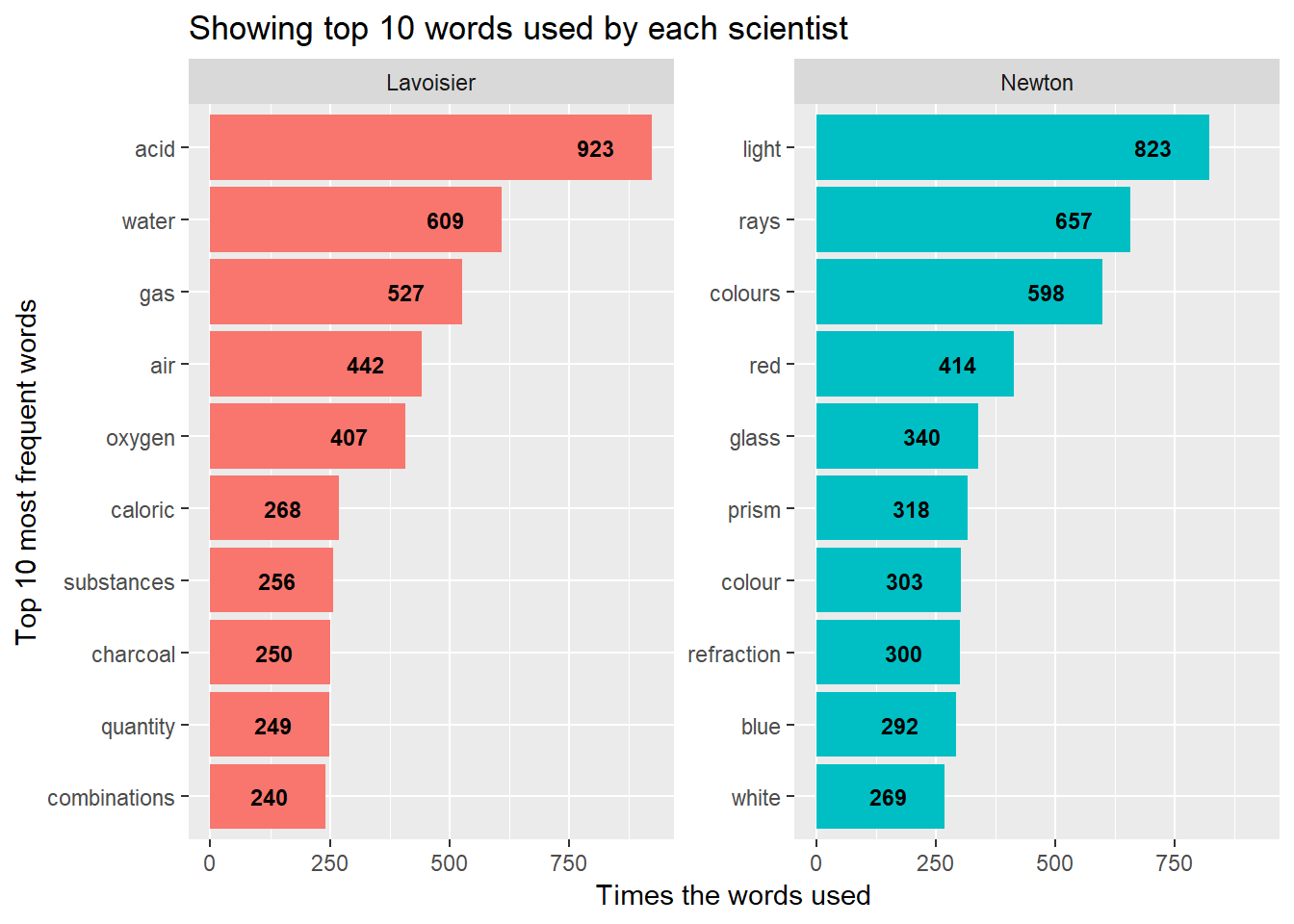
You can see by looking at words used by these 2 scientists, how the words encompass 2 subjects area. Words like acid, gas, oxygen define these came from subject as Chemistry while words like light, rays, prism show they are from Physics.
Now lets dive into more analysis. As I above mentioned, I’m going to use 3 methods to separate out words from these 2 books.
1. Log Odds Ratio
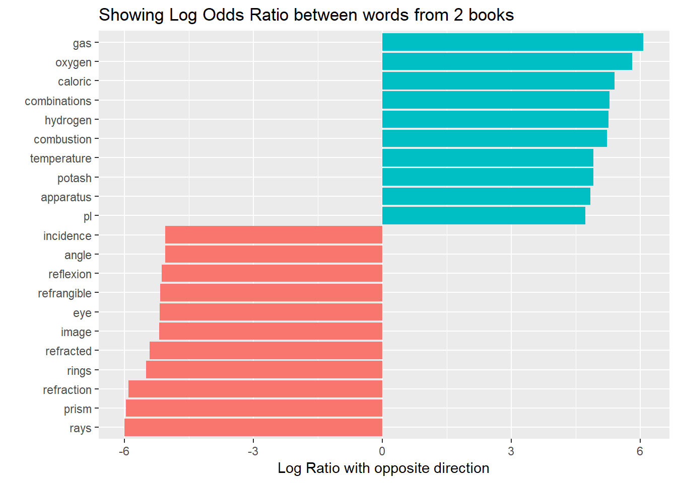
Log odds ratio is a statistical tool to find out the probability of happening one event out of 2 events. In our case, its finding out which words are more or less likely to come from each book.

Here n is number of times that word is used by each scientist and total is total words by each one of them. Let’s turn this equation into code and print out again 10 top words from each book.
by_words %>%
  spread(scientist,n, fill = 0) %>%
  mutate_if(is.numeric, funs((.+1)/(sum(.+1)))) %>%
  mutate(logratio = log(Lavoisier/Newton)) %>%
  group_by(logratio>0) %>%
  top_n(10, abs(logratio)) %>%
  ungroup() %>%
  mutate(word = fct_reorder(word, logratio)) %>%
  ggplot(aes(word, logratio, fill = logratio > 0))+
  geom_col(show.legend = FALSE)+
  coord_flip()+
  labs(title = "Showing Log Odds Ratio between words from 2 books",
       x= "",
       y = "Log Ratio with opposite direction")
Again its clearly visible how words are distinct from one subject to the other.
2. tf-idf
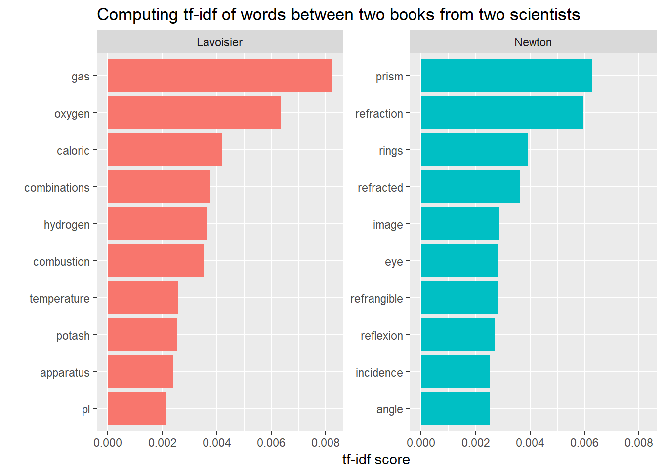
As Julia Silge defines tf-idf is a heuristic approach to identify certain words out of collection of documents. It helps to find out those words which are specific to a particular documents. This method relies on method called Inverse Document Frequency, which can be explained as below.

When this term is multiplied by term frequency, frequency of terms in a document, then we have tf-idf
Again lets convert these into code and find out result to visualise.
by_words %>%
  bind_tf_idf(word,scientist,n) %>%
  group_by(scientist) %>%
  top_n(10, tf_idf) %>%
  ungroup() %>%
  mutate(word = fct_reorder(word, tf_idf)) %>%
  ggplot(aes(word, tf_idf, fill = scientist))+
  geom_col(show.legend = FALSE)+
  coord_flip()+
  facet_wrap(~scientist, scales = "free_y")+
  labs(title = "Computing tf-idf of words between two books from two scientists",
       x= "",
       y = "tf-idf score")
We find similar result with this approach too.
3. Weighted Log Odds
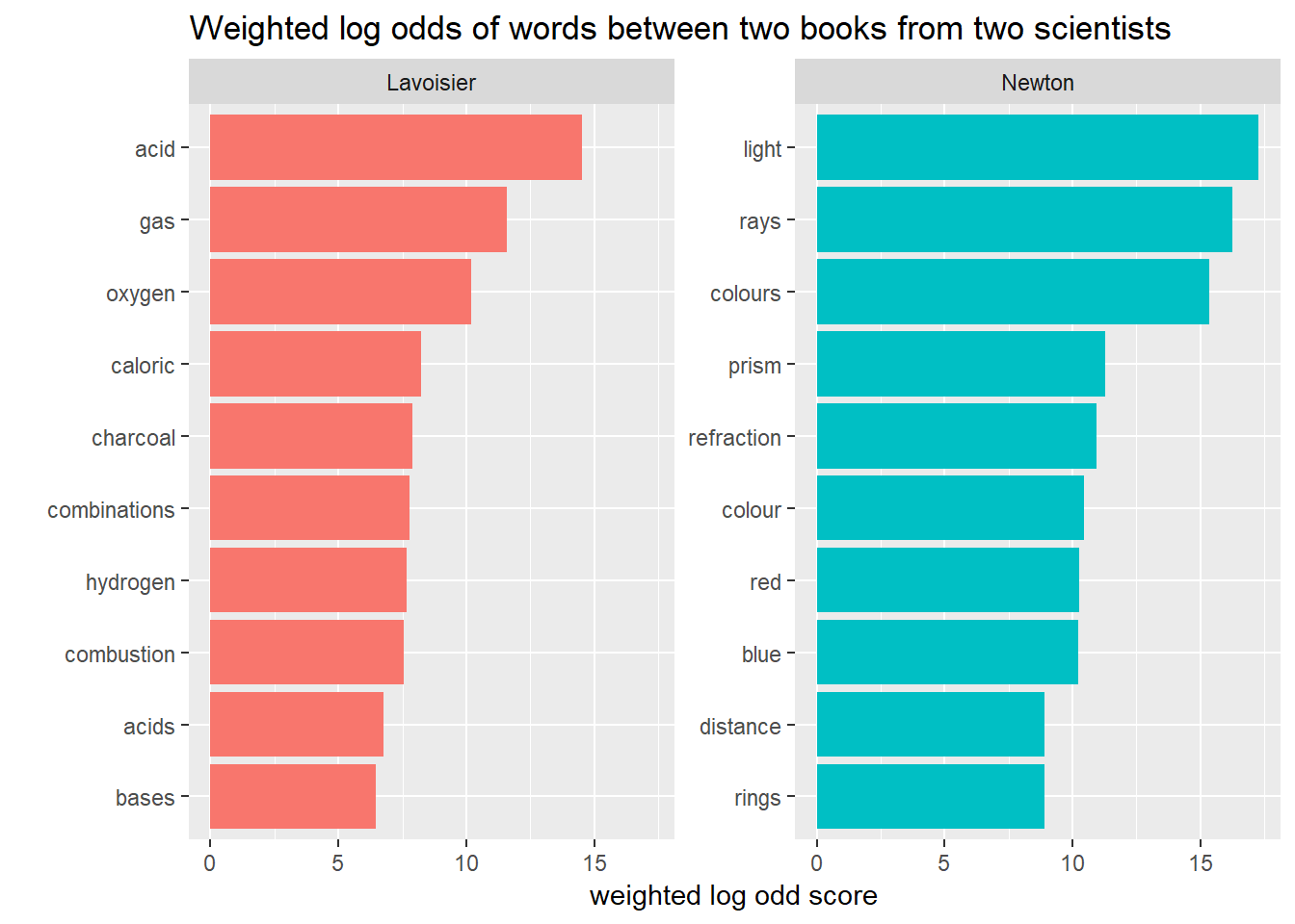
This approach is recently introduced by Julia Silge and her colleague. As the author suggested, when the counts of number of features are different, this method works better than old Log odds ratio. They argue this methods accounts for Sampling Variability. Let’s put this into our code and find out the result.
by_words %>%
  bind_log_odds(scientist,word, n) %>%
  group_by(scientist) %>%
  top_n(10, log_odds) %>%
  ungroup() %>%
  mutate(word = fct_reorder(word, log_odds)) %>%
  ggplot(aes(word, log_odds, fill = scientist))+
  geom_col(show.legend = FALSE)+
  coord_flip()+
  facet_wrap(~scientist, scales = "free_y")+
  labs(title = "Weighted log odds of words between two books from two scientists",
       x= "",
       y = "weighted log odd score")
This method also gives similar results as other methods.
Conclusion
We explored 3 methods to isolate and extract a set of words which are completely different from one another in terms of subject they represent. We have these 3 methods in our disposal to move ahead into Topic Modelling. You can find more about this by referring to Julia Silge’s blog. Another place where you will have tons of treasure is Text mining with R
