Topic Modelling In R
In this post I’m doing some topic modelling. Topic modelling is a way of finding abstact topics in collection of documents. I’m using Sherlock Holmes stories and try to find out which word contributes to how much in telling what the story is about. One way to think about is certain words will play important role in defining what the story is about and the frequncy of those words play vital role in our task.
I’m using gutenbergr package to download 12 Sherlock Holmes stories.
sherlock_raw<-gutenberg_download(1661)

sherlock<-sherlock_raw %>%
  mutate(story = ifelse(str_detect(text,"ADVENTURE"),text,NA),
         line = row_number()) %>%
  fill(story) %>%
  filter(story!= "THE ADVENTURES OF SHERLOCK HOLMES")
Few steps are done to prepare the data but still out data is not in tidy format so let tidy it.
sherlock_tidy<-sherlock %>%
  unnest_tokens(word,text) %>%
  anti_join(stop_words) %>%
  filter(!word %in% c("holmes", "sherlock", "HOLMES", "SHERLOCK"))
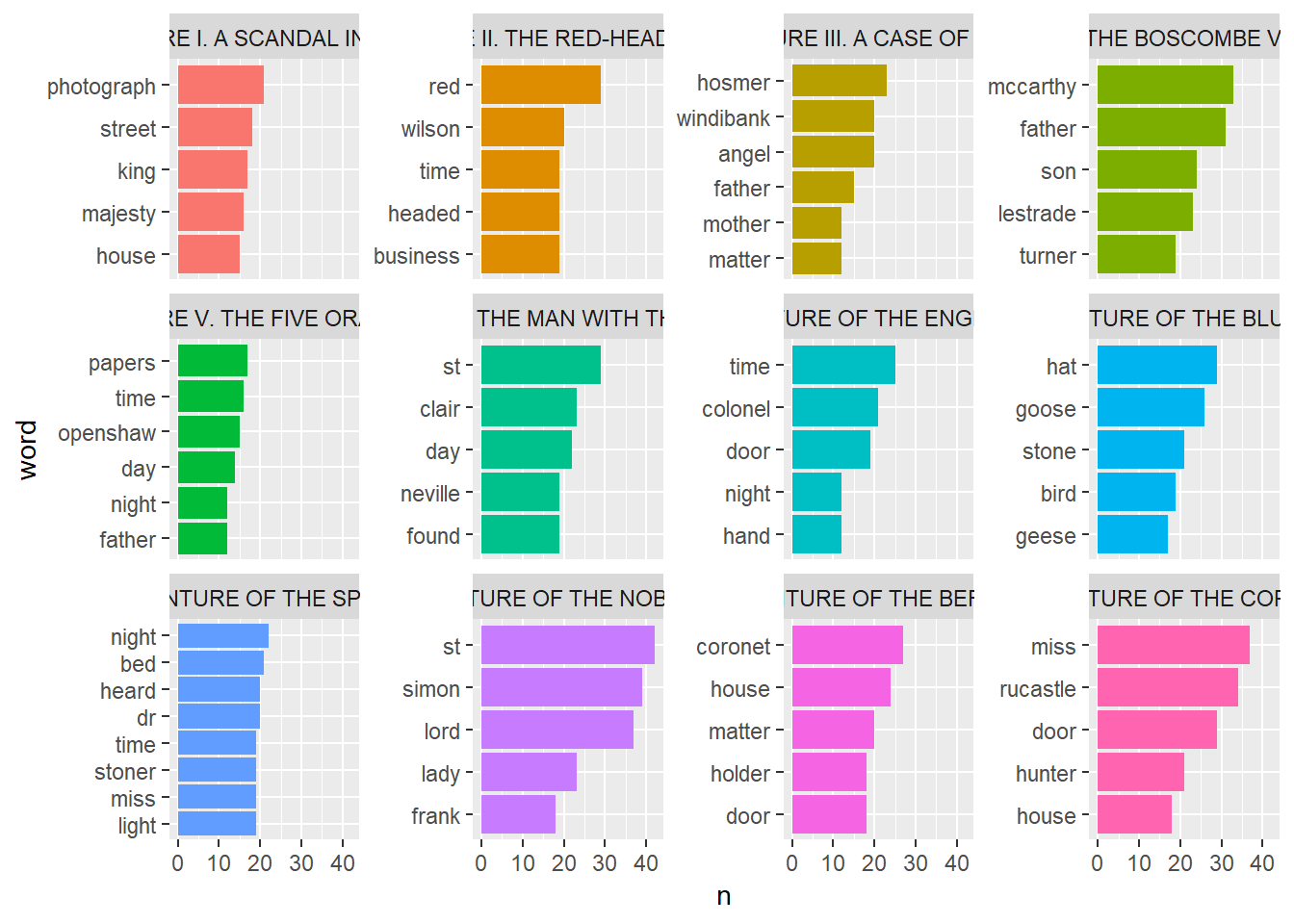
One of the ways to know what a document is by analysing most frequently used words. Here I’m finding 5 most frequently used words in each of the story. Its called Term Frequency (tf).
top_5_words<-sherlock_tidy %>%
  count(story, word) %>%
  #arrange(-n) %>%
  group_by(story) %>%
  top_n(5) %>%
  ungroup()
top_5_words
## # A tibble: 65 x 3
## story word n
## <chr> <chr> <int>
## 1 ADVENTURE I. A SCANDAL IN BOHEMIA house 15
## 2 ADVENTURE I. A SCANDAL IN BOHEMIA king 17
## 3 ADVENTURE I. A SCANDAL IN BOHEMIA majesty 16
## 4 ADVENTURE I. A SCANDAL IN BOHEMIA photograph 21
## 5 ADVENTURE I. A SCANDAL IN BOHEMIA street 18
## 6 ADVENTURE II. THE RED-HEADED LEAGUE business 19
## 7 ADVENTURE II. THE RED-HEADED LEAGUE headed 19
## 8 ADVENTURE II. THE RED-HEADED LEAGUE red 29
## 9 ADVENTURE II. THE RED-HEADED LEAGUE time 19
## 10 ADVENTURE II. THE RED-HEADED LEAGUE wilson 20
## # ... with 55 more rowswe can visualize our results.
top_5_words %>%
  mutate(word = reorder_within(word,n,story)) %>%
  ggplot(aes(word,n, fill=story))+
  geom_col(show.legend = FALSE)+
  facet_wrap(~story, scales = "free_y")+
  scale_x_reordered() +
  coord_flip()
By going through frequency of words we will find lots of words within each story but they are less significant on telling us what the story is all about. Yet one another sophisticated method is knowing the
 Inverse Document Frequency (idf) of words. Its natural log of ratio between number of documents divided by number of documents containing that word.
Suppose, a word is found in all the documents, then this ratio becomes 1 and natural log of 1 is 0. So all the words which are present in most of the documents will have low value. This shows those words are not suitable to describe as they will generalize our result. But if a word is only available in one or two documents, then its value will be higher as the ratio will be less than 1 and natural log of that value will be greater than 0.
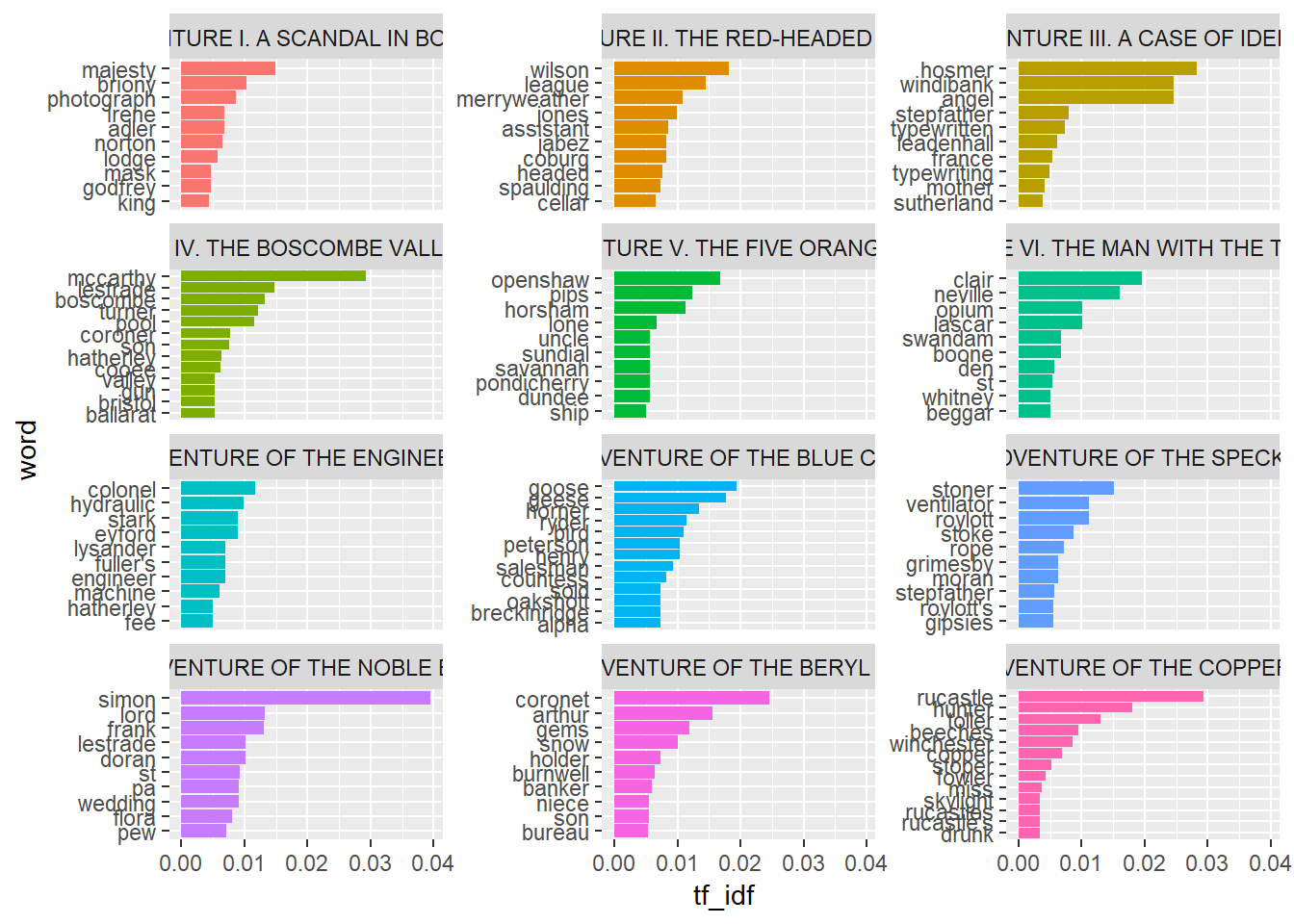
In Tidytext package we have bind_tf_idf function which we can use to calculate tf_idf this value. tf_idf is product of Term Frequency (tf) and Inverse Document Frequency (idf). We can find 10 top words from each docments which are unique to only one of each and visualise the result.
sherlock_tf_idf<-sherlock_tidy %>%
  count(story,word,sort = TRUE) %>%
  bind_tf_idf(word,story,n) %>%
  arrange(-tf_idf) %>%
  group_by(story) %>%
  top_n(10) %>%
  ungroup
sherlock_tf_idf
## # A tibble: 129 x 6
## story word n tf idf tf_idf
## <chr> <chr> <int> <dbl> <dbl> <dbl>
## 1 X. THE ADVENTURE OF THE NOBLE BACHE~ simon 39 0.0159 2.48 0.0394
## 2 XII. THE ADVENTURE OF THE COPPER BE~ rucastle 34 0.0118 2.48 0.0293
## 3 ADVENTURE IV. THE BOSCOMBE VALLEY M~ mccarthy 33 0.0118 2.48 0.0292
## 4 ADVENTURE III. A CASE OF IDENTITY hosmer 23 0.0114 2.48 0.0283
## 5 ADVENTURE III. A CASE OF IDENTITY angel 20 0.00991 2.48 0.0246
## 6 ADVENTURE III. A CASE OF IDENTITY windiba~ 20 0.00991 2.48 0.0246
## 7 XI. THE ADVENTURE OF THE BERYL CORO~ coronet 27 0.00990 2.48 0.0246
## 8 ADVENTURE VI. THE MAN WITH THE TWIS~ clair 23 0.00785 2.48 0.0195
## 9 VII. THE ADVENTURE OF THE BLUE CARB~ goose 26 0.0108 1.79 0.0194
## 10 XII. THE ADVENTURE OF THE COPPER BE~ hunter 21 0.00729 2.48 0.0181
## # ... with 119 more rowssherlock_tf_idf %>%
mutate(word = reorder_within(word,tf_idf,story)) %>%
ggplot(aes(word,tf_idf, fill=story))+
geom_col(show.legend = FALSE)+
facet_wrap(~story, scales = "free_y", ncol = 3)+
scale_x_reordered() +
coord_flip() So these words can show in someway what each story is about. Now we are going to do some topic modelling.
Topic Modelling
We are using stm package to do topic modelling. First we have to convert our tidy data into Document Term Matrix
sherlock_dfm<-sherlock_tidy %>%
  count(story,word,sort = TRUE) %>%
  cast_dfm(story,word,n)
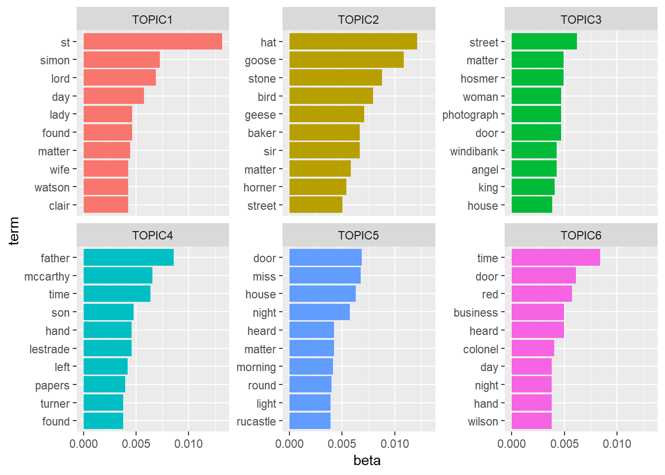
We are trining our model with 6 topics. And we are using tidy function to define our output of our model. First we calculate `Beta’ value it defines per-topic-per-word probability.
sherlock_model<-stm(sherlock_dfm, K = 6,init.type = "Spectral",verbose = FALSE)

top_10_beta<-tidy(sherlock_model) %>%
  arrange(-beta) %>%
  group_by(topic) %>%
  top_n(10,beta) %>%
  ungroup

top_10_beta
## # A tibble: 60 x 3
## topic term beta
## <int> <chr> <dbl>
## 1 1 st 0.0132
## 2 2 hat 0.0121
## 3 2 goose 0.0108
## 4 2 stone 0.00876
## 5 4 father 0.00856
## 6 6 time 0.00838
## 7 2 bird 0.00793
## 8 1 simon 0.00724
## 9 2 geese 0.00709
## 10 5 door 0.00687
## # ... with 50 more rowsHere if we just isolate word ‘st’ and try to see its beta distribution, we can see the respective probabilities of the word being in each topic.
tidy(sherlock_model) %>%
  filter(term == "st") %>%
  arrange(-beta)
## # A tibble: 6 x 3
## topic term beta
## <int> <chr> <dbl>
## 1 1 st 1.32e- 2
## 2 3 st 1.28e- 3
## 3 6 st 5.71e- 4
## 4 2 st 4.16e- 4
## 5 4 st 1.98e- 4
## 6 5 st 2.64e-30Now let’s visualize this result.
top_10_beta %>%
  mutate(term = reorder_within(term,beta,topic),
         topic = paste0("TOPIC", topic)) %>%
  ggplot(aes(term,beta, fill=topic))+
  geom_col(show.legend = FALSE)+
  facet_wrap(~topic, scales = "free_y", ncol = 3)+
  scale_x_reordered() +
  coord_flip()
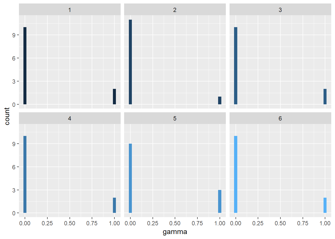
There is one more distribution called ‘gamma’. Its per-document-per-topic probability. Lets calculate and vizualise the result.
sherlock_gamma<-tidy(sherlock_model, matrix = "gamma", document_names = rownames(sherlock_dfm))sherlock_gamma %>%
ggplot(aes(gamma, fill= topic))+
geom_histogram(show.legend = FALSE)+
facet_wrap(~topic) It shows which document belongs to which topic.
Conclusion
Topic Modelling is a vast subject. There are more into it like Topic Modelling using ‘ngrams’. Please refer to great post by Julia Silgie
